Multiple Plots in MATLAB

In the last two tutorial posts, we discussed the basics of MATLAB plots and different options for formatting MATLAB plots. We will now go one step further and find out how to create multiple plots in MATLAB. Specifically, I will introduce how to create multiple plots lines on one axis and how to create lines on different axes within the same figure. Both of these arrangements are extremely useful in engineering when we wish to show multiple sets of related data!

Multiple MATLAB Plots on One Axis

There are different ways to create multiple lines on the same set of axes. I'm going introduce the way I usually do it using the hold function, which I feel gives the most control over the output. I'd like to demonstrate this by example as before where I will first give the code, then describe it below.

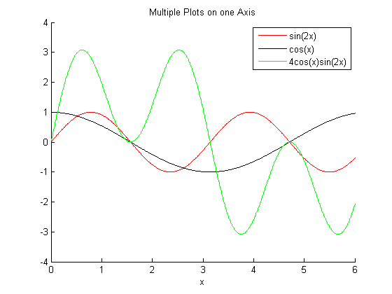
Lets assume we would like to plot three functions , , and for zero to 6 on the same set of axes. MATLAB code that will do this is given as

% Create vector of x data
x = [0:0.01:6];
% Evaluate equations element-by-element
y1 = sin(2*x);
y2 = cos(x);
y3 = 4*cos(x).*sin(2*x);
 
% Create a new figure and turn "hold on"
figure
hold on
plot(x,y1,'r')
plot(x,y2,'k')
plot(x,y3,'g')
     title('Multiple Plots on one Axis')
     xlabel('x')
     legend('sin(2x)','cos(x)','4cos(x)sin(2x)')

In the code we first create a vector for x and evaluate the three functions we wish to plot. Next we create a figure window with figure function and immediately after we use the command hold on - this tells MATLAB to put all of the plots from this point forward into the current figure window.

Note that we then simply create each plot in the usual way. I use multiple colors here to differentiate the lines from one another (if we don't do this all lines will default to blue).

Finally, I use another new function to include a legend on the plot. The legend function takes a series of string inputs to describe the lines on the plot. The first input to legend corresponds to the first plot() function used in the figure, the second input to the second plot(), and so on. You can include as many inputs to legend as you need to describe all of the lines in the figure; however, you must input them in the proper order.

The figure resulting from the previous code is given below.

MATLAB Plots on Multiple Axes

We could also plot the above functions on different axes using the subplot() function in MATLAB. The subplot() function is used to tell MATLAB how to split up the figure window and where to place the graph from each successive plot() command.

Below shows MATLAB code for how to plot the functions on three separate axes. A description of how subplot() is used immediately follows.

% Create the vector of x data
x = [0:0.01:6];
% Evaluate the equations for y
y1 = sin(2*x);
y2 = cos(x);
y3 = 4*cos(x).*sin(2*x);
 
% Create a new figure window
figure
% Create the first subplot within the figure (location 3,1,1 - top)
subplot(3,1,1)
    plot(x,y1,'r')
    xlabel('x')
    ylabel('sin(2x)')
% Create the second subplot within the figure (location 3,1,2 - middle)
subplot(3,1,2)
    plot(x,y2,'k')
    xlabel('x')
    ylabel('cos(x)')
% Create the third subplot within the figure (location 3,1,3 - bottom)
subplot(3,1,3)
    plot(x,y3,'g')
    xlabel('x')
    ylabel('4cos(x)sin(2x)')

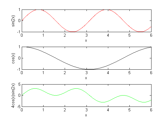
We note above that subplot() has three inputs with the first two being identical each time it is used. The first two inputs tell MATLAB how to split the figure up. Imagine it as how many "rows" and "columns" of plots there will be in the figure. In the example above, our figure will have three rows of plots and one column.

The third input to subplot() tells MATLAB in what location to place the graph from the next plot() command. This value will change depending on the number of rows and columns for the plot. To figure it out, you simply count first across the columns and down the rows. Here our indices one through three are simply counted down the rows since there is only one column.

Thinking about a more complex example, if we wanted a figure with three rows and two columns of plots and a specific plot to go into the second row and second column would be given by subplot(3,2,4). It goes into the fourth index based on counting across columns in the first row as 1 and 2, then columns in the the second row giving index 3 and 4.

We also note that within each subplot() we can specify individual axis labels and graph titles as shown in the sample code. The figure resulting from are example is given below.